TL;DR

The following learning notes try to give some intuition on how Stable Diffusion works, some mathematical intuition on Diffusion Models and an introduction to Latent Diffusion Models.

The following sources were extensively used during creation of this learning notes. Passages may be reutilized to create a reasonable overview of the topic. Credit goes to the authors of the following papers and posts.

Illustrations by Jay Alammar

Sohl-Dickstein et al., 2015

Ho et al. 2020

Rombach & Blattmann, et al. 2022

Lilian Weng on Diffusion Models

Sergios Karagiannakos on Diffusion Models

Hugging Face on Annotated Diffusion Model

If you recently introduced yourself to strangers and told them about your job in AI, there is a good chance they asked you about the current hype-train around the next generation of generative AI models and related data products like Dall-E, Stable Diffusion or Midjourney.

Latent Diffusion Models like the ones above had some significant media attention. While no one outside AI community bats an eye if Deepmind creates an algorithm, that beats the (almost ancient) and important Strassen-Algorithm by some percent in computation complexity(which is a tremendous progress), nearly everyone is excited to create made up pictures of cats doing crazy stuff through a simple interface.

Stable Diffusion “cat surfing waves at sunset, comic style”

While those models already made a name for themselves by winning art competitions, are adopted by companies into their related data products(Canva.com, Shutterstock.com) and start-ups creating those products raising billions in venture capital you may ask yourself:

What is all the fuzz about?
What is behind the hype? What are Latent Diffusion Models?
What is the math behind them?
Do they impact my life? What is the best way to leverage their power?

Let me briefly introduce you to Diffusion Models and Latent Diffusion Models and explain the math.

If you are interested in a Hands-On you can find that in my other post:

Hands on Latent Diffusion Models

If you want an awesome visual introduction with diagrams i strongly advise to visit the blog by Jay Alammar.

What is this post about:

A brand-new category of cutting-edge generative models called diffusion models generate a variety of high-resolution images. They have already received a great deal of attention as a result of OpenAI, Nvidia, and Google’s success in training massive models. We’ll take a deeper look into Denoising Diffusion Probabilistic Models (also known as DDPMs, diffusion models, score-based generative models or simply autoencoders) as researchers have been able to achieve remarkable results with them for (un)conditional image/audio/video generation. Popular examples (at the time of writing) include GLIDE and DALL-E 2 by OpenAI, Latent Diffusion by the University of Heidelberg and ImageGen by Google Brain.

Intuition on Diffusion Models

You may ask “What is the intuition behind diffusion models?” Let’s break it down with a short example to make it clear: You are a painter hired by Vatican with the task to repaint the fresco at the ceiling of sixtinian chapel.

The requirement is to recreate the fresco with pictures of cats. The requirement is based on the old fresco and the vatican wants to have the same scenes as currently there but witch cats. So you start remembering the fresco and start bringing up a base coat and the old fresco soon becomes a big grey noise.

Most likely you will be overwhelmed with creating a big fresco and immediately think of structuring your work into smaller chunks. Then you may outline the structures you want to paint based on your memory on the old picture and your vision on the new one.

Maybe you start with one object like the arm of Adam, from the creation of Adam and then focus on the hand. Gradually you add more details and finally are happy with the scene, decide to finish it and tackle the next part. Still later you may change things after you decided that it fits better with the overall fresco.

Finally you are building a masterpiece lasting centuries until someone thinks dogs are nicer than cats(so never).

The same idea comes with Diffusion: Gradually add noise and create the best representation of the input vision in many small steps. Breaking up the image sampling allows the models to correct itself over those small steps iteratively and produces a good sample.

Unfortunately nothing is cost-neutral. Like it will cost a painter like Michealangelo almost 4 years to finish the fresco in Sixtinian chapel, the iterative process makes the Models slow at sampling(At least compared to GANs).

What are Diffusion Models?

The idea of diffusion for generative modeling was introduced in (Sohl-Dickstein et al., 2015). However, it took until (Song et al., 2019) (at Stanford University), and then (Ho et al., 2020) (at Google Brain) who independently improved the approach. DDPM which we are focussing on originally was introduced in a paper by (Ho et al., 2020).

At a high level, they work by first representing the input signal as a set of latent variables, which are then transformed through a series of probabilistic transformations to produce the output signal. The transformation process is designed to smooth out the noise in the input signal and reconstruct a cleaner version of the signal.

Transformation consist of 2 processes.

In a bit more detail for images, the set-up consists of 2 processes:

a fixed (or predefined) forward diffusion process $q$ of our choosing, that gradually adds Gaussian noise to an image, until you end up with pure noise
a learned reverse denoising diffusion process $p_\theta$, where a neural network is trained to gradually denoise an image starting from pure noise, until you end up with an actual image.

Diffusion Models are basically generative models: 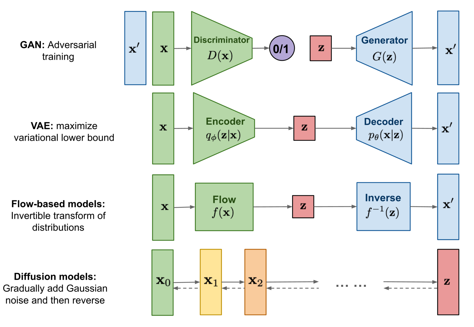Overview of the different types of generative models

I want to see the math

Diffusion

In probability theory and statistics, diffusion processes are a class of continuous-time Markov process with almost surely continuous sample paths. E.g. Brownian motion

Wikipedia says:

A Markov chain or Markov process is a stochastic model describing a sequence of possible events in which the probability of each event depends only on the state attained in the previous event.
A continuous-time Markov chain (CTMC) is a continuous stochastic process in which, for each state, the process will change state according to an exponential random variable and then move to a different state as specified by the probabilities of a stochastic matrix

Diffusion consists of 2 processes:

a fixed (or predefined) forward diffusion process $q$ of our choosing, that gradually adds Gaussian noise to an image, until you end up with pure noise
a learned reverse denoising diffusion process $p_\theta$, where a neural network is trained to gradually denoise an image starting from pure noise, until you end up with an actual image.

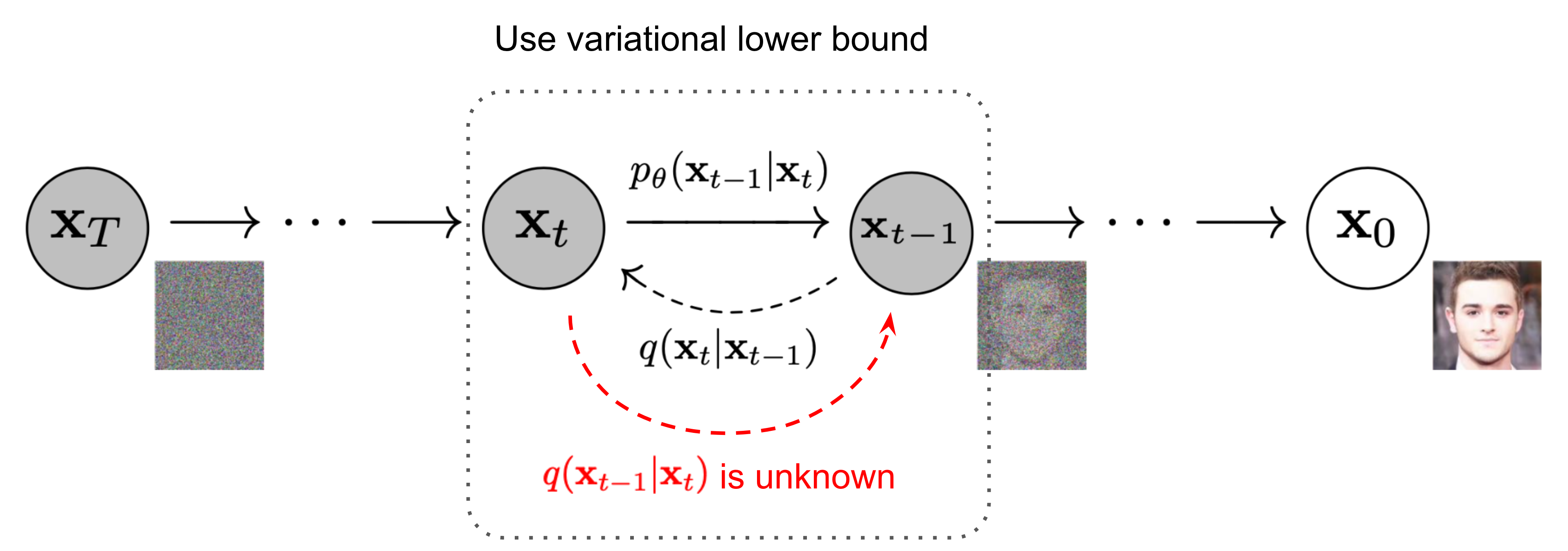DDPM The Markov chain of forward (reverse) diffusion process of generating a sample by slowly adding (removing) noise. (Image source: Ho et al. 2020) and Lilian Weng

Forward Diffusion

Given a data point from a real data distribution $x_0 \sim q(x)$ we define a forward diffusion in which we add small Gaussian noise stepwise for $T$ steps producing noisy samples $\mathbf{x}_1, \dots, \mathbf{x}_T$

Step sizes are controlled by a variance schedule $0 < \beta_1 < \beta_2 < … < \beta_T < 1$.

It is defined as

$q(x_t | x_{t-1}) = \mathcal{N}(x_t; \sqrt{1 - \beta_t} x_{t-1}, \beta_t \mathbf{I})$ with $\sqrt{1 - \beta_t} x_{t-1}$ as decay towards origin and

$\beta_t \mathbf{I}$ as the addition of small noise.

Rephrased: A normal distribution (also called Gaussian distribution) is defined by 2 parameters:

a mean $\mu$ and
a variance $\sigma^2 \geq 0$.

Basically, each new (slightly noisier) image at time step $t$ is drawn from a conditional Gaussian distribution with

$\mathbf{\mu}_t = \sqrt{1 - \beta_t} \mathbf{x}_{t-1}$ and
$\sigma^2_t = \beta_t$,

which we can do by sampling $\mathbf{\epsilon} \sim \mathcal{N}(0, \mathbf{I})$ and then setting $\mathbf{x}_t = \sqrt{1 - \beta_t} \mathbf{x}_{t-1} + \sqrt{\beta_t} \mathbf{\epsilon}$.

Given a sufficiently large $T$ and a well behaved schedule for adding noise at each time step, you end up with what is called an isotropic Gaussian distribution at $t=T$ via a gradual process.

Isotropic means the probability density is equal (iso) in every direction (tropic). In gaussians this can be achieved with a $\sigma^2 I$ covariance matrix.

One property of the diffusion process is, that you can sample $x_t$ at any time step $t$ using reparameterization trick. Let $\alpha_{t} = 1 - \beta_t$ and $\bar{\alpha}_t = \prod_{i=1}^t \alpha_i$

$$ \begin{aligned} \mathbf{x}_t &= \sqrt{\alpha_t}\mathbf{x}_{t-1} + \sqrt{1 - \alpha_t}\boldsymbol{\epsilon}_{t-1} & \text{ ;where } \boldsymbol{\epsilon}_{t-1}, \boldsymbol{\epsilon}_{t-2}, \dots \sim \mathcal{N}(\mathbf{0}, \mathbf{I}) \\ &= \sqrt{\alpha_t}\mathbf{x}_{t-1} + \sqrt{1 - \alpha_t}\boldsymbol{\epsilon}_{t-1} & \text{ ;where } \boldsymbol{\epsilon}_{t-1}, \boldsymbol{\epsilon}_{t-2}, \dots \sim \mathcal{N}(\mathbf{0}, \mathbf{I}) \\ &= \sqrt{\alpha_t \alpha_{t-1}} \mathbf{x}_{t-2} + \sqrt{1 - \alpha_t \alpha_{t-1}} \bar{\boldsymbol{\epsilon}}_{t-2} & \text{ ;where } \bar{\boldsymbol{\epsilon}}_{t-2} \text{ merges two Gaussians.} \\ &= \dots \\ &= \sqrt{\bar{\alpha}_t}\mathbf{x}_0 + \sqrt{1 - \bar{\alpha}_t}\boldsymbol{\epsilon}\\ q(\mathbf{x}_t \vert \mathbf{x}_0) &= \mathcal{N}(\mathbf{x}_t; \sqrt{\bar{\alpha}_t} \mathbf{x}_0, (1 - \bar{\alpha}_t)\mathbf{I}) \end{aligned} $$

So the sampling of noise and creation of $x_t$ is done in one step only and can be sampled at any timestep.

Reverse Diffusion

$q(x_{t-1} \vert x_t)$ which denotes the Reverse Process is intractable since statistical estimates of it require computations involving the entire dataset and therefore we need to learn a model $p_0$ to approximate these conditional probabilities in order to run the reverse diffusion process.

We need to learn a model $p_0$ to approximate these conditional probabilities

Since $q(x_{t-1} \vert x_t)$ will also be Gaussian, for small enough $\beta_t$, we can choose $p_0$ to be Gaussian and just parameterize the mean and variance as the Reverse Diffusion:

$\quad p_\theta(\mathbf{x}_{t-1} \vert \mathbf{x}_t) = \mathcal{N} (\mathbf{x}_{t-1}; {\mu}_\theta(\mathbf{x}_t, t), {\Sigma}_\theta(\mathbf{x}_t, t)) $

with $\mu_\theta(x_{t},t)$ as the mean and $\Sigma_\theta (x_{t},t)$ as the variance

conditioned on the noise level $t$ as the to be learned functions of drift and covariance of the Gaussians(by a Neural Net).

As the target image is already defined the problem can be described as a supervised learning problem.

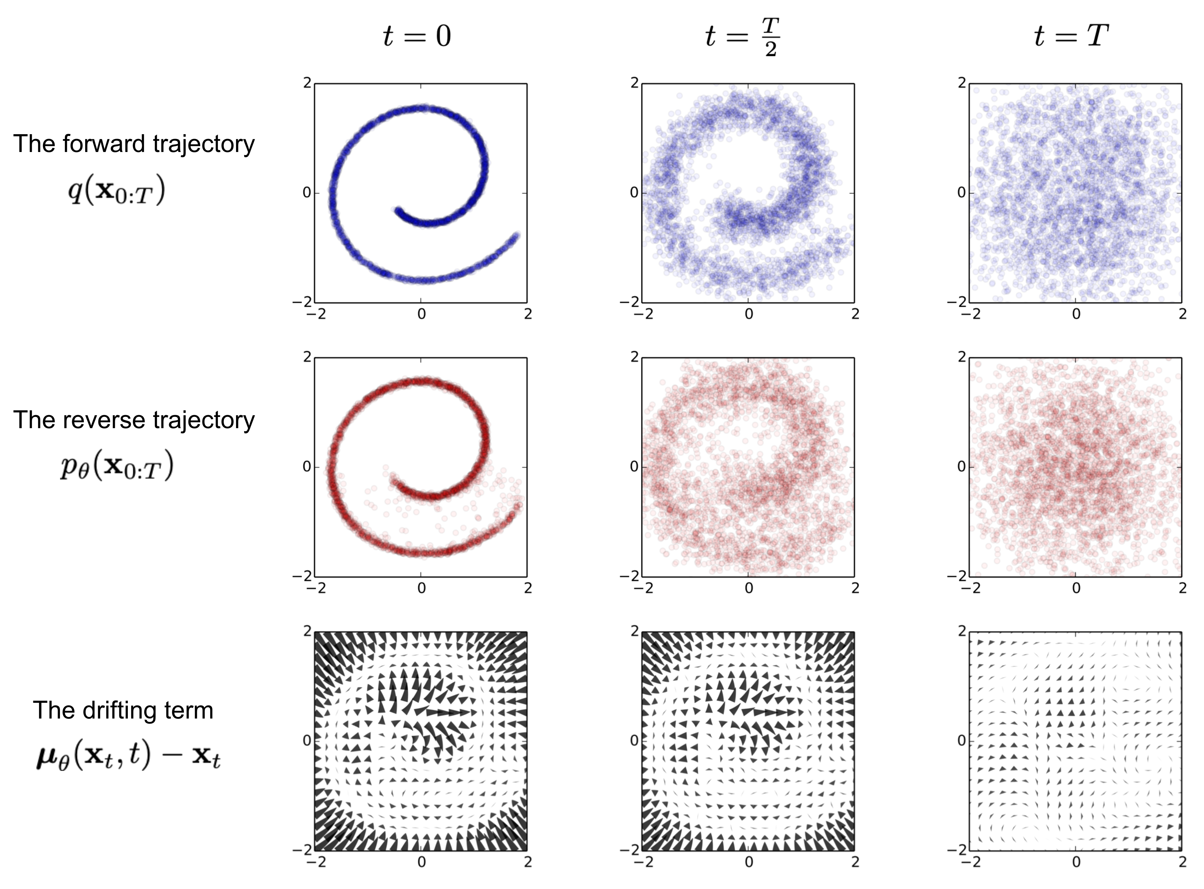
An example of training a diffusion model for modeling a 2D swiss roll data. (Image source: Sohl-Dickstein et al., 2015)

Hence, our neural network needs to learn/represent the mean and variance. However, the DDPM authors decided to keep the variance fixed, and let the neural network only learn (represent) the mean $\mu_\theta$ of this conditional probability distribution.

Optimization of the Loss Function

To derive an objective function to learn the mean of the backward process, the authors observe that the combination of $q$ and $p_\theta$ can be seen as a variational auto-encoder (VAE) (Kingma et al., 2013).

A Diffusion Model can be trained by finding the reverse Markov transitions that maximize the likelihood of the training data. In practice, training equivalently consists of minimizing the variational upper bound on the negative log likelihood

$- \log p_\theta(\mathbf{x}_0)$.

After transformation(Lilian Weng for reference), we can write the evidence lower bound (ELBO) as follows:

$$ \begin{aligned} - \log p_\theta(\mathbf{x}_0) &\leq - \log p_\theta(\mathbf{x}_0)+ D_\text{KL}(q(\mathbf{x}_{1:T}\vert\mathbf{x}_0) \vert p_\theta(\mathbf{x}_{1:T}\vert\mathbf{x}_0) ) \end{aligned} $$

Intuition on the optimization: For a function $f(x)$, which can’t be computed(like e.g. the above negative log-likelihood) and have also a function $g(x)$, which we can compute and fullfills the condition $g(x) <= f(x)$. If we then maximize $g(x)$ we can be certain that $f(x)$ will also increase.

For optimization we use Kullback-Leibler (KL) Divergences. The KL Divergence is a statistical distance measure of how much one probability distribution $P$ differs from a reference distribution $Q$.

We are interested in formulating the Loss function in terms of KL divergences because the transition distributions in our Markov chain are Gaussians, and the KL divergence between Gaussians has a closed form. For a closer look please look here

If we rewrite the above Loss function and apply the bayesian rule the upper term can be summarized to a joint probability and will be trainsformed to the Variational Lower Bound:

$$ \begin{aligned} &= -\log p_\theta(\mathbf{x}_0) + \mathbb{E}_{\mathbf{x}_{1:T}\sim q(\mathbf{x}_{1:T} \vert \mathbf{x}_0)} \Big[ \log\frac{q(\mathbf{x}_{1:T}\vert\mathbf{x}_0)}{p_\theta(\mathbf{x}_{0:T}) / p_\theta(\mathbf{x}_0)} \Big] \\ &= -\log p_\theta(\mathbf{x}_0) + \mathbb{E}_q \Big[ \log\frac{q(\mathbf{x}_{1:T}\vert\mathbf{x}_0)}{p_\theta(\mathbf{x}_{0:T})} + \log p_\theta(\mathbf{x}_0) \Big] \\ &= \mathbb{E}_q \Big[ \log \frac{q(\mathbf{x}_{1:T}\vert\mathbf{x}_0)}{p_\theta(\mathbf{x}_{0:T})} \Big] \\ \text{Let }L_\text{VLB} &= \mathbb{E}_{q(\mathbf{x}_{0:T})} \Big[ \log \frac{q(\mathbf{x}_{1:T}\vert\mathbf{x}_0)}{p_\theta(\mathbf{x}_{0:T})} \Big] \geq - \mathbb{E}_{q(\mathbf{x}_0)} \log p_\theta(\mathbf{x}_0) \end{aligned} $$

Complete calculation can be found here together with a really nice explanation here

The objective can be further rewritten to be a combination of several KL-divergence and entropy terms(Detailed process in Appendix B in Sohl-Dickstein et al., 2015)

$$ \begin{aligned} L_\text{VLB} &= \mathbb{E}_{q(\mathbf{x}_{0:T})} \Big[ \log\frac{q(\mathbf{x}_{1:T}\vert\mathbf{x}_0)}{p_\theta(\mathbf{x}_{0:T})} \Big] \\ &= \dots \\ &= \mathbb{E}_q [\underbrace{D_\text{KL}(q(\mathbf{x}_T \vert \mathbf{x}_0) \parallel p_\theta(\mathbf{x}_T))}_{L_T} + \sum_{t=2}^T \underbrace{D_\text{KL}(q(\mathbf{x}_{t-1} \vert \mathbf{x}_t, \mathbf{x}_0) \parallel p_\theta(\mathbf{x}_{t-1} \vert\mathbf{x}_t))}_{L_{t-1}} \underbrace{- \log p_\theta(\mathbf{x}_0 \vert \mathbf{x}_1)}_{L_0} ] \end{aligned} $$

Reshaped:

$$ \begin{aligned} L_\text{VLB} &= L_T + L_{T-1} + \dots + L_0 \\ \text{where } L_T &= D_\text{KL}(q(\mathbf{x}_T \vert \mathbf{x}_0) \parallel p_\theta(\mathbf{x}_T)) \\ L_t &= D_\text{KL}(q(\mathbf{x}_t \vert \mathbf{x}_{t+1}, \mathbf{x}_0) \parallel p_\theta(\mathbf{x}_t \vert\mathbf{x}_{t+1})) \text{ for }1 \leq t \leq T-1 \\ L_0 &= - \log p_\theta(\mathbf{x}_0 \vert \mathbf{x}_1) \end{aligned} $$

Every KL term in $L_\text{VLB}$ except for $L_0$ compares two Gaussian distributions and therefore they can be computed in closed form. $L_T$ is constant and can be ignored during training because $q$ has no learnable parameters and $x_T$ is a Gaussian noise. $L_t$ formulates the difference between the desired denoising steps and the approximated ones.

It is evident that through the ELBO, maximizing the likelihood boils down to learning the denoising steps $L_t$.

We would like to train $\boldsymbol{\mu}_\theta$ to predict $\tilde{\boldsymbol{\mu}}_t = \frac{1}{\sqrt{\alpha_t}} \Big( \mathbf{x}_t - \frac{1 - \alpha_t}{\sqrt{1 - \bar{\alpha}_t}} \boldsymbol{\epsilon}_t \Big)$. Because $\mathbf{x}_t$ is available as input at training time, we can reparameterize the Gaussian noise term instead to make it predict $\boldsymbol{\epsilon}_t$ from the input $\mathbf{x}_t$ at time step $t$:

$$ \begin{aligned} \boldsymbol{\mu}_\theta(\mathbf{x}_t, t) &= \color{red}{\frac{1}{\sqrt{\alpha_t}} \Big( \mathbf{x}_t - \frac{1 - \alpha_t}{\sqrt{1 - \bar{\alpha}_t}} \boldsymbol{\epsilon}_\theta(\mathbf{x}_t, t) \Big)} \\ \text{Thus }\mathbf{x}_{t-1} &= \mathcal{N}(\mathbf{x}_{t-1}; \frac{1}{\sqrt{\alpha_t}} \Big( \mathbf{x}_t - \frac{1 - \alpha_t}{\sqrt{1 - \bar{\alpha}_t}} \boldsymbol{\epsilon}_\theta(\mathbf{x}_t, t) \Big), \boldsymbol{\Sigma}_\theta(\mathbf{x}_t, t)) \end{aligned} $$

The loss term $L_t$ is parameterized to minimize the difference from $\tilde\mu$ :

$$ \begin{aligned} L_t &= \mathbb{E}_{\mathbf{x}_0, \boldsymbol{\epsilon}} \Big[\frac{1}{2 | \boldsymbol{\Sigma}_\theta(\mathbf{x}_t, t) |^2_2} | \color{blue}{\tilde{\boldsymbol{\mu}}_t(\mathbf{x}_t, \mathbf{x}_0)} - \color{green}{\boldsymbol{\mu}_\theta(\mathbf{x}_t, t)} |^2 \Big] \\ &= \mathbb{E}_{\mathbf{x}_0, \boldsymbol{\epsilon}} \Big[\frac{1}{2 |\boldsymbol{\Sigma}_\theta |^2_2} | \color{blue}{\frac{1}{\sqrt{\alpha_t}} \Big( \mathbf{x}_t - \frac{1 - \alpha_t}{\sqrt{1 - \bar{\alpha}_t}} \boldsymbol{\epsilon}_t \Big)} - \color{green}{\frac{1}{\sqrt{\alpha_t}} \Big( \mathbf{x}_t - \frac{1 - \alpha_t}{\sqrt{1 - \bar{\alpha}_t}} \boldsymbol{\boldsymbol{\epsilon}}_\theta(\mathbf{x}_t, t) \Big)} |^2 \Big] \\ &= \mathbb{E}_{\mathbf{x}_0, \boldsymbol{\epsilon}} \Big[\frac{ (1 - \alpha_t)^2 }{2 \alpha_t (1 - \bar{\alpha}_t) | \boldsymbol{\Sigma}_\theta |^2_2} |\boldsymbol{\epsilon}_t - \boldsymbol{\epsilon}_\theta(\mathbf{x}_t, t)|^2 \Big] \\ &= \mathbb{E}_{\mathbf{x}_0, \boldsymbol{\epsilon}} \Big[\frac{ (1 - \alpha_t)^2 }{2 \alpha_t (1 - \bar{\alpha}_t) | \boldsymbol{\Sigma}_\theta |^2_2} |\boldsymbol{\epsilon}_t - \boldsymbol{\epsilon}_\theta(\sqrt{\bar{\alpha}_t}\mathbf{x}_0 + \sqrt{1 - \bar{\alpha}_t}\boldsymbol{\epsilon}_t, t)|^2 \Big] \end{aligned} $$

The final objective function $L_t$ then looks as follows (for a random time step $t$ given $\mathbf{\epsilon} \sim \mathcal{N}(\mathbf{0}, \mathbf{I})$ ) as shown by Ho et al. (2020)

$$ | \mathbf{\epsilon} - \mathbf{\epsilon}_\theta(\mathbf{x}_t, t) |^2 = | \mathbf{\epsilon} - \mathbf{\epsilon}_\theta( \sqrt{\bar{\alpha}_t} \mathbf{x}_0 + \sqrt{(1- \bar{\alpha}_t) } \mathbf{\epsilon}, t) |^2.$$

Here, $\mathbf{x}_0$ is the initial (real, uncorrupted) image, and we see the direct noise level $t$ sample given by the fixed forward process. $\mathbf{\epsilon}$ is the pure noise sampled at time step $t$, and $\mathbf{\epsilon}_\theta (\mathbf{x}_t, t)$ is our neural network. The neural network is optimized using a simple mean squared error (MSE) between the true and the predicted Gaussian noise.

The training algorithm now looks as follows:

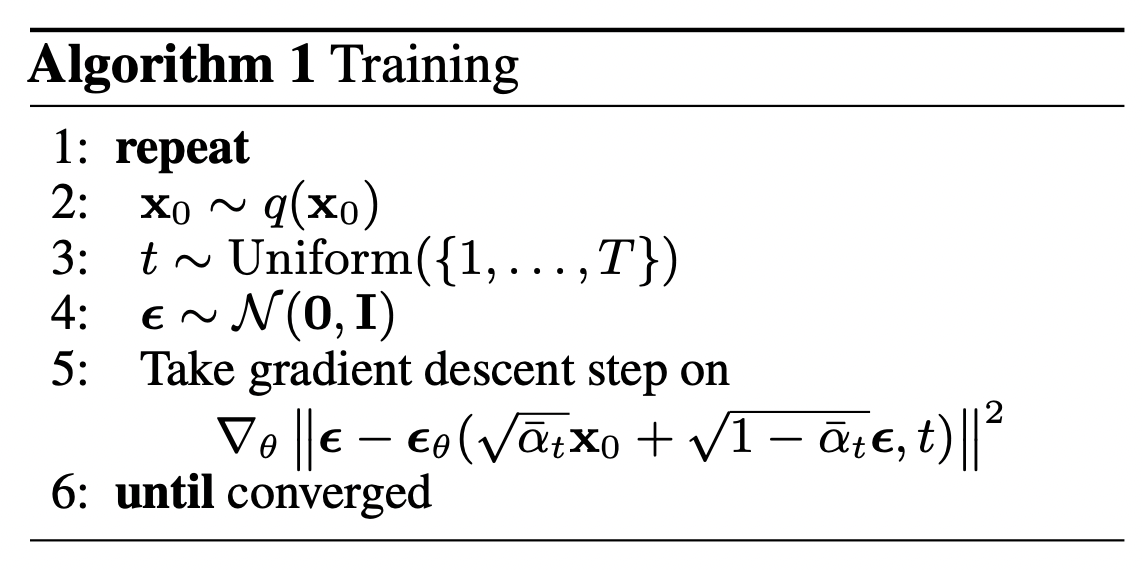
In other words:

we take a random sample $\mathbf{x}_0$ from the real unknown and possibily complex data distribution $q(\mathbf{x}_0)$
we sample a noise level $t$ uniformally between $1$ and $T$ (i.e., a random time step)
we sample some noise from a Gaussian distribution and corrupt the input by this noise at level $t$ (using the nice property defined above)
the neural network is trained to predict this noise based on the corrupted image $\mathbf{x}_t$ (i.e. noise applied on $\mathbf{x}_0$ based on known schedule $\beta_t$ )

Neural Nets

The neural network needs to take in a noised image at a particular time step and return the predicted noise. Note that the predicted noise is a tensor that has the same size/resolution as the input image. So technically, the network takes in and outputs tensors of the same shape. What type of neural network can we use for this?

What is typically used here is very similar to that of an Autoencoder, which you may remember from typical “intro to deep learning” tutorials. Autoencoders have a so-called “bottleneck” layer in between the encoder and decoder. The encoder first encodes an image into a smaller hidden representation called the “bottleneck”, and the decoder then decodes that hidden representation back into an actual image. This forces the network to only keep the most important information in the bottleneck layer.

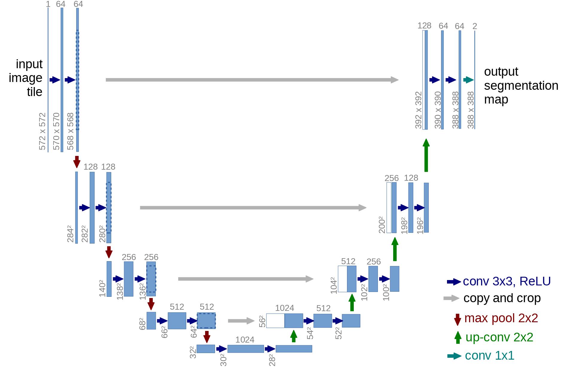
In terms of architecture, the DDPM authors went for a U-Net, introduced by (Ronneberger et al., 2015) (which, at the time, achieved state-of-the-art results for medical image segmentation). This network, like any autoencoder, consists of a bottleneck in the middle that makes sure the network learns only the most important information. Importantly, it introduced residual connections between the encoder and decoder, greatly improving gradient flow (inspired by ResNet in He et al., 2015).

The math on Latent Diffusion

It is very slow to generate a sample from DDPM by following the Markov chain of the reverse diffusion process, as can be up to one or a few thousand steps. One data point from Song et al. 2020: “For example, it takes around 20 hours to sample 50k images of size 32 × 32 from a DDPM, but less than a minute to do so from a GAN on an Nvidia 2080 Ti GPU.”

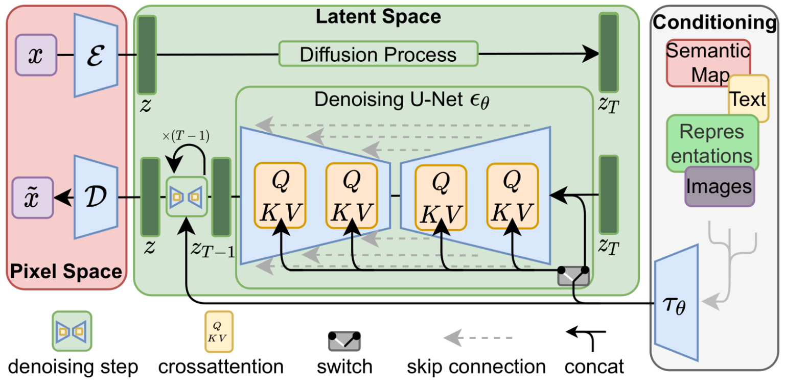
Latent diffusion model (LDM; Rombach & Blattmann, et al. 2022) runs the diffusion process in the latent space instead of pixel space, making training cost lower and inference speed faster. It is motivated by the observation that most bits of an image contribute to perceptual details and the semantic and conceptual composition still remains after aggressive compression. LDM loosely decomposes the perceptual compression and semantic compression with generative modeling learning by first trimming off pixel-level redundancy with autoencoder and then manipulate/generate semantic concepts with diffusion process on learned latent.

It is motivated by the observation that most bits of an image contribute to perceptual details and the semantic and conceptual composition still remains after aggressive compression.

LDM loosely decomposes the perceptual compression and semantic compression with generative modeling learning by first trimming off pixel-level redundancy with autoencoder and then manipulate/generate semantic concepts with diffusion process on learned latent.

The perceptual compression process relies on an autoencoder model.

An encoder $\mathcal{E}$ is used to compress the input image $\mathbf{x} \in \mathbb{R}^{H \times W \times 3}$ to a smaller 2D latent vector $\mathbf{z} = \mathcal{E}(\mathbf{x}) \in \mathbb{R}^{h \times w \times c}$ , where the downsampling rate $f=H/h=W/w=2^m, m \in \mathbb{N}$.

Then an decoder $\mathcal{D}$ reconstructs the images from the latent vector, $\tilde{\mathbf{x}} = \mathcal{D}(\mathbf{z})$.

The paper explored two types of regularization in autoencoder training to avoid arbitrarily high-variance in the latent spaces.

KL-reg: A small KL penalty towards a standard normal distribution over the learned latent, similar to VAE.
VQ-reg: Uses a vector quantization layer within the decoder, like VQVAE but the quantization layer is absorbed by the decoder.

The diffusion and denoising processes happen on the latent vector $\mathbf{z}$. The denoising model is a time-conditioned U-Net, augmented with the cross-attention mechanism to handle flexible conditioning information for image generation (e.g. class labels, semantic maps, blurred variants of an image).

The design is equivalent to fuse representation of different modality into the model with cross-attention mechanism.

Each type of conditioning information is paired with a domain-specific encoder $\tau_\theta$ to project the conditioning input $y$ to an intermediate representation that can be mapped into cross-attention component, $\tau_\theta(y) \in \mathbb{R}^{M \times d_\tau}$:

$$ \begin{aligned} &\text{Attention}(\mathbf{Q}, \mathbf{K}, \mathbf{V}) = \text{softmax}\Big(\frac{\mathbf{Q}\mathbf{K}^\top}{\sqrt{d}}\Big) \cdot \mathbf{V} \\ &\text{where }\mathbf{Q} = \mathbf{W}^{(i)}_Q \cdot \varphi_i(\mathbf{z}_i),; \mathbf{K} = \mathbf{W}^{(i)}_K \cdot \tau_\theta(y),; \mathbf{V} = \mathbf{W}^{(i)}_V \cdot \tau_\theta(y) \\ &\text{and } \mathbf{W}^{(i)}_Q \in \mathbb{R}^{d \times d^i_\epsilon},; \mathbf{W}^{(i)}_K, \mathbf{W}^{(i)}_V \in \mathbb{R}^{d \times d_\tau},; \varphi_i(\mathbf{z}_i) \in \mathbb{R}^{N \times d^i_\epsilon},; \tau_\theta(y) \in \mathbb{R}^{M \times d_\tau} \end{aligned} $$

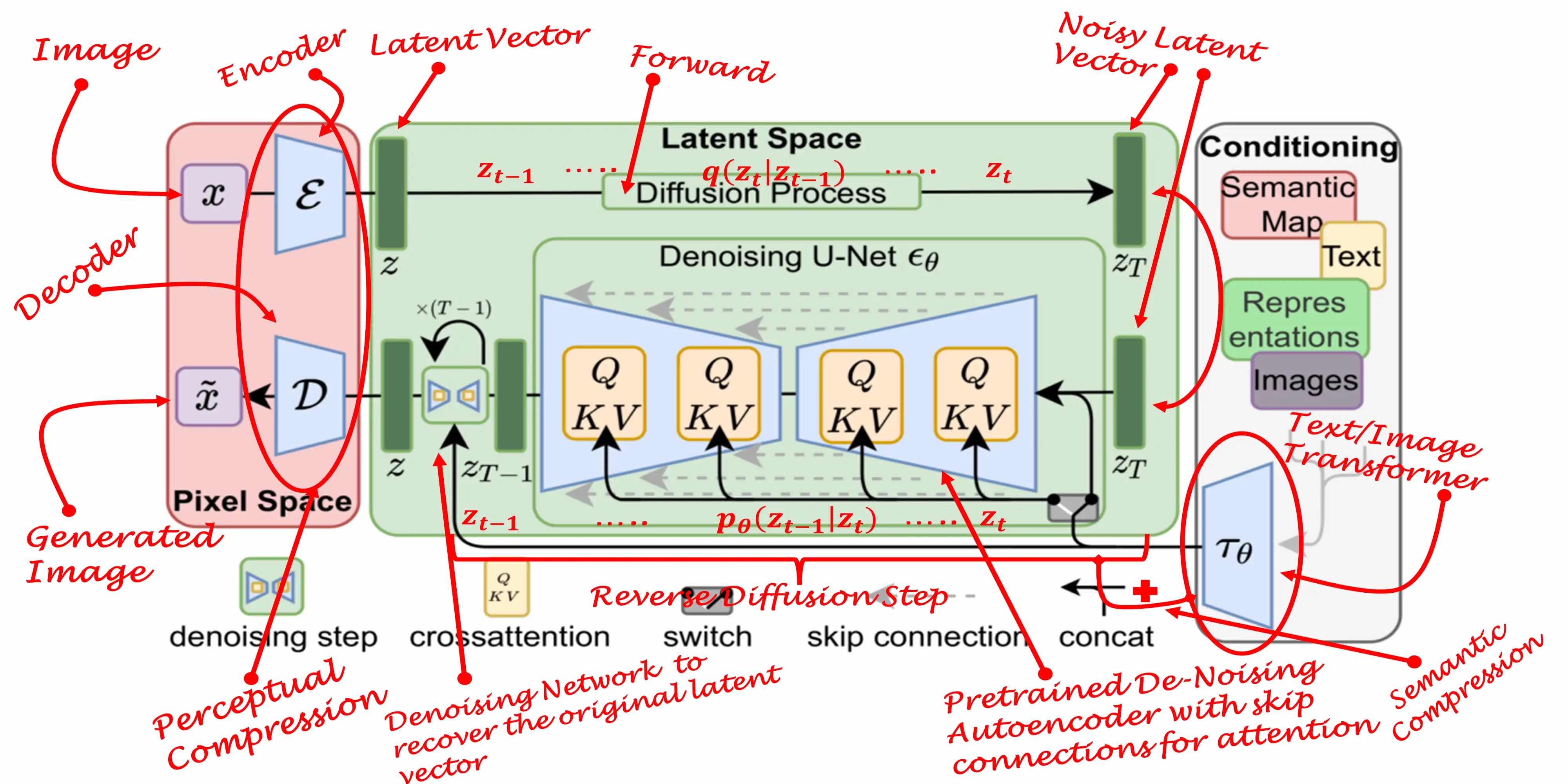Picture from J. Rafid Siddiqui